 Coaching Centre
Processing and graphing data
Building results tables with trials and means, types of data, choosing the right graph including histograms and scatter graphs, lines of best fit and outliers, calculating and interpreting a gradient, interpolation and extrapolation, and using spreadsheets.
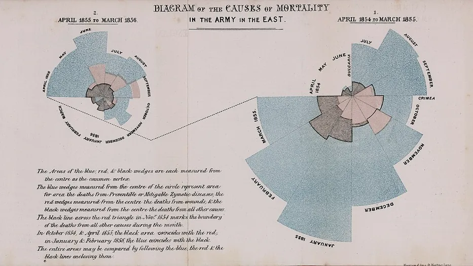
In the Crimean War in the 1850s, British army hospitals were losing far more soldiers to infections like cholera and typhus than to battle wounds, but tables of numbers in official reports didn't move anyone. Florence Nightingale, a nurse trained in statistics, redrew the data as a new kind of graph: a circle of wedges, one for each month, coloured by cause of death. The enormous blue wedges for preventable disease made the problem impossible to ignore, and helped win reforms in hospital sanitation. The right graph can make data speak.
Results tables
Raw data goes in your logbook as you measure it. For the report, build a clear table:
- A numbered, descriptive title naming both variables ("Table 1: Mass of water lost from pots with different mulches over 7 days").
- The independent variable in the first column, then each trial, then the calculated mean.
- Units in the column headings only, in brackets: "Mass lost (g)".
- The same number of decimal places throughout a column, matching the instrument's resolution.
- A dash (–) for missing data, with a note explaining why, and outliers marked rather than deleted.
| Mulch type | Pot 1 (g) | Pot 2 (g) | Pot 3 (g) | Pot 4 (g) | Mean mass lost (g) |
|---|---|---|---|---|---|
| None (control) | 218.4 | 209.7 | 216.2 | 211.9 | 214.1 |
| Sugarcane | 98.1 | 92.6 | 95.0 | 98.3 | 96.0 |
| Pine bark | 121.3 | 113.8 | 119.6 | 117.5 | 118.1 |
| Gravel | 149.2 | 153.8 | 201.5* | 150.4 | 151.1 |
* Pot 3 was knocked over on day 4 and lost soil (see logbook p. 17). It was excluded from the mean and repeated afterwards.
Types of data
- Qualitative (categorical): names or categories, such as mulch type or eye colour.
- Quantitative discrete: counts that can only be whole numbers, such as number of seeds germinated.
- Quantitative continuous: measurements that can take any value in a range, such as mass, temperature or time.
The type of data decides the type of graph.
Choosing a graph
You met column and line graphs in Year 7 (1H). Two more are useful in research projects:
- A histogram shows how often values of one continuous variable fall in each range (class), such as the lengths of 60 oysters. The bars touch because the scale is continuous.
- A scatter graph plots pairs of measurements, such as the height and arm span of each student, to see whether two variables are related. You add a line of best fit if there is a trend.
Lines of best fit and outliers
Measured data always has scatter, so never join the dots. Draw a single straight line or smooth curve that follows the trend, with points scattered evenly on both sides. It doesn't have to pass through any particular point, including the origin, unless you know it must.
An outlier is a point well away from the trend. Don't just delete it. Check your logbook for a reason (a spill, a misread scale), repeat that measurement if you can, and leave the outlier out of the line of best fit only if you have a good reason, saying so in your report. Sometimes an "outlier" is the most interesting result in the whole project.
Gradient: what the slope tells you
The gradient (slope) of a straight line of best fit tells you how fast the dependent variable changes as the independent variable increases:
gradient = rise ÷ run = change in y ÷ change in x
A pea seedling is measured each day: 2.1, 3.0, 4.1, 4.6, 5.8, 6.0 and 7.8 cm on days 0 to 6. Find its growth rate from the line of best fit.
Always give the gradient its units (units of y ÷ units of x) and say what it means. On a distance–time graph it is the speed; on a mass–volume graph it is the density; on a rate-of-reaction graph it is the rate. A gradient taken from a line of best fit uses all the data, so it is more reliable than a value calculated from any single pair of readings.
Interpolation means reading a value from the line within the range of your data (the pea was about 5.2 cm tall at day 3.5). Extrapolation means extending the line beyond your data, which is risky: the pea won't keep growing at 0.89 cm per day forever.
Using a spreadsheet
Spreadsheets save time and mistakes. Type raw data in columns, use =AVERAGE() for means and =MAX()−MIN() for ranges, and insert a scatter chart with a trendline (which can show the gradient). But check what the software does: spreadsheets often join dots, choose odd scales, leave off axis titles, or offer 3D charts that distort the data. You are responsible for the graph, not the program.
- Find all four problems in the mulch depth graph, then show the fixed version. Which problem would change the shape of the curve the most?
- In the paper towel graph, how much better does Brand C look than Brand A before and after the fix?
- In the cooling water graph, why is the dashed extrapolation physically impossible?
- Which mistakes do you think spreadsheet software would make for you automatically?
Test yourself
Which graph best shows the lengths of 80 fish caught in a survey, grouped into 5 cm ranges?
One continuous variable grouped into ranges: a histogram.
A line of best fit on a distance–time graph passes through (2 s, 6 m) and (10 s, 30 m). The gradient is
(30 − 6) ÷ (10 − 2) = 24 ÷ 8 = 3 m/s.
Where should units appear in a results table?
Units go in the headings so the cells contain only numbers.
Reading a value from a line of best fit beyond the range of the data is called
Extrapolation assumes the trend continues, which it may not.
Label the parts of the graph.
Which graph suits each data set?
A point far from the trend is an . The slope of a line of best fit is its . Reading a value between data points is . Data that can only be whole numbers is . Bars touch on a .
A student measures the extension of a spring for masses of 0, 50, 100, 150, 200 and 250 g and gets 0, 2.1, 3.9, 9.5, 8.2 and 10.1 cm. Describe how the student should graph these results and find the spring's extension per gram, and explain how they should deal with the reading at 150 g.
Both variables are continuous, so the student should draw a scatter (line) graph with mass (g), the independent variable, on the x-axis and extension (cm) on the y-axis, both with even scales, labelled with units, and a title. After plotting the points, they should draw a single straight line of best fit, not join the dots. The reading at 150 g (9.5 cm) is an outlier: the other points rise by about 2 cm for every 50 g, so about 6 cm is expected. The student should check their logbook for a reason, such as misreading the ruler, and repeat that measurement. If no repeat is possible, they should leave the point on the graph but draw the line through the other points, and explain this in the report. The line should pass through (0, 0) and close to (250, 10.1). Using two points on the line far apart, gradient = (10.0 − 0) ÷ (250 − 0) = 0.040 cm per gram, so the spring stretches about 0.04 cm, or 4 cm per 100 g.